Analysing survey data with complex sampling in R

The is the final session of the workshop and covers a few extensions, including regression diagnostics.

Load packages

Load all of the required packages if they are not already in your R environment.

Load data

Remember that we “saved” our wrangled dataset to the working directory in the previous section as an .RDatafile in our workshop folder.

Code

root <- "C://Users//s1769862//OneDrive - University of Edinburgh//SLTF-workshop-August2024//" # change with where the folder lies in your filepath
ess9 <- readRDS(file= file.path(root, "Data", "ess9.RData"))

We also need to re-specify our sampling design object and PSU adjustment settings.

Code

design2 <- survey::svydesign(ids = ~psu, strata = ~stratum, weights = ~anweight, data = ess9)
options(survey.lonely.psu="adjust") # adjust for lonely psu

Model fit

First, we can expand upon the reporting of regression outputs by integrating model fit criteria into the summary tables.

This can be accomplished via glance table from the gtsummary tbl_regression function, which pulls the fit information directly from the svyglm model output.

Code

survey::svyglm(nwspol ~ age, family=gaussian, design=design2) %>%
  tbl_regression() %>%
  bold_p(t=0.05) %>%
  add_glance_table(include=c(everything()))

Characteristic	Beta	95% CI¹	p-value
age
18 to 25	—	—
25 to 35	5.1	-5.8, 16	0.4
36 to 49	3.9	-6.0, 14	0.4
50 to 64	17	6.5, 28	0.002
65+	39	30, 49	<0.001
Null deviance	1,315,576,458
Null df	47,593
AIC	614,789
BIC	1,305,684,998
Deviance	1,305,684,944
Residual df	21,255
No. Obs.	47,594
¹ CI = Confidence Interval

This also applied to logistic regression results

Code

survey::svyglm(vote ~ trstprl + gender + age, family=quasibinomial, design = design2) %>% tbl_regression(exponentiate=T, label = c(trstprl~"Trust in parliament")) %>%
  bold_p(t=0.05) %>%
  add_glance_table(include=c(everything()))

Characteristic	OR¹	95% CI¹	p-value
Trust in parliament	1.17	1.15, 1.19	<0.001
gender
Female	—	—
Male	1.04	0.96, 1.12	0.4
age
18 to 25	—	—
25 to 35	1.43	1.24, 1.66	<0.001
36 to 49	2.06	1.79, 2.37	<0.001
50 to 64	3.01	2.61, 3.47	<0.001
65+	3.41	2.95, 3.94	<0.001
Null deviance	44,668
Null df	44,077
AIC	42,547
BIC	42,587
Deviance	42,512
Residual df	19,811
No. Obs.	44,078
¹ OR = Odds Ratio, CI = Confidence Interval

Pseudo r-squared

The automatic summary output does not include a pseudo r-squared estimate, but we can request this manually from the survey package.

Code

m1 <- survey::svyglm(vote ~ trstprl + gender + age, family=quasibinomial, design = design2)
psrsq(m1)

[1] 0.04923396

We can add this information back to our the summary object created for the model.

Code

m1$r.squared <- psrsq(m1)

m1 %>% tbl_regression(exponential=T,label = c(trstprl~"Trust in parliament")) %>%
  bold_p(t=0.05) %>%
  add_glance_table(include=c(everything()))

Characteristic	log(OR)¹	95% CI¹	p-value
Trust in parliament	0.16	0.14, 0.17	<0.001
gender
Female	—	—
Male	0.04	-0.04, 0.11	0.4
age
18 to 25	—	—
25 to 35	0.36	0.21, 0.51	<0.001
36 to 49	0.72	0.58, 0.86	<0.001
50 to 64	1.1	0.96, 1.2	<0.001
65+	1.2	1.1, 1.4	<0.001
Null deviance	44,668
Null df	44,077
AIC	42,547
BIC	42,587
Deviance	42,512
Residual df	19,811
No. Obs.	44,078
¹ OR = Odds Ratio, CI = Confidence Interval

Note

You can select which estimation methods to use! See the full list on the data documentation methods = c("Nagelkerke", "Cox-Snell")

Task 9

Add model fit information to your own regression model.

Customise the output information and styling!
For reference, see tbl_regression

Code

## Write your own code!

Plotting model coefficients

Model coefficients from survey adjusted models can also be plotted.

I like using the jtools package for visualising the odds rations from binary logistic regression models.

Code

survey::svyglm(vote ~ trstprl + gender + age, family=quasibinomial, design = design2) %>%
  jtools::plot_coefs(exp=T,
                     coefs = c("Trust in parliament" = "trstprl",
                               "Gender(ref=male)" = "genderMale",
                               "Age 25-35(ref=18-25)" = "age25 to 35",
                               "Age 36-49(ref=18-25)" = "age36 to 49",
                               "Age 50-64(ref=18-25)" = "age50 to 64",
                               "Age 65+(ref=18-25)" = "age65+"))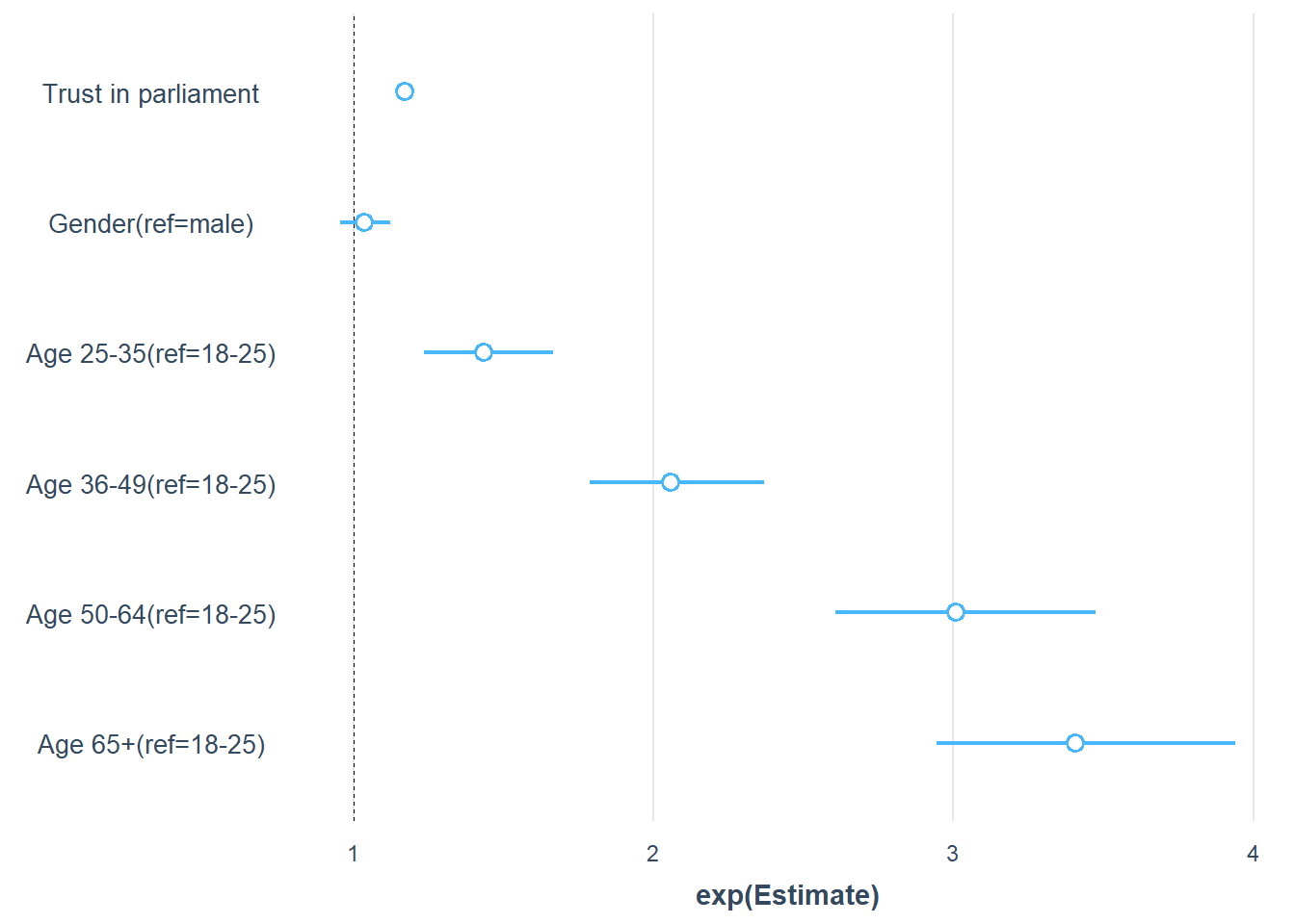

Plotting predicted values

Beyond coefficients, predicted values can be plotted and evaluated.

Let us go back and create a model for predicting news consumption using OLS regression to see effect plots for continuous outcomes.

I theorise that trust is parliament is predictive of increased news consumption, and wish to control for age and gender.

Code

m2 <- survey::svyglm(nwspol ~ age + gender + trstprl, family=gaussian, design=design2)

We can go back and look at the model summary.

Code

m2 %>%
  tbl_regression(exponential=T,label = c(trstprl~"Trust in parliament")) %>%
  add_glance_table(include=c(everything())) %>%
  bold_p(t=0.05)

Characteristic	Beta	95% CI¹	p-value
age
18 to 25	—	—
25 to 35	5.4	-5.9, 17	0.4
36 to 49	3.9	-6.1, 14	0.4
50 to 64	17	6.2, 28	0.002
65+	40	31, 50	<0.001
gender
Female	—	—
Male	8.0	2.9, 13	0.002
Trust in parliament	0.38	-0.83, 1.6	0.5
Null deviance	1,269,936,326
Null df	46,606
AIC	599,723
BIC	1,259,242,848
Deviance	1,259,242,773
Residual df	20,956
No. Obs.	46,607
¹ CI = Confidence Interval

It looks like my predicted relationship is not supported by the model.

Nevertheless, we can investigate the model fit and predicted values.

First, we can use an effect plot to look at the predicted relationship between trust in parliament and news consumption.

Code

jtools::effect_plot(m2, pred=trstprl, interval = T)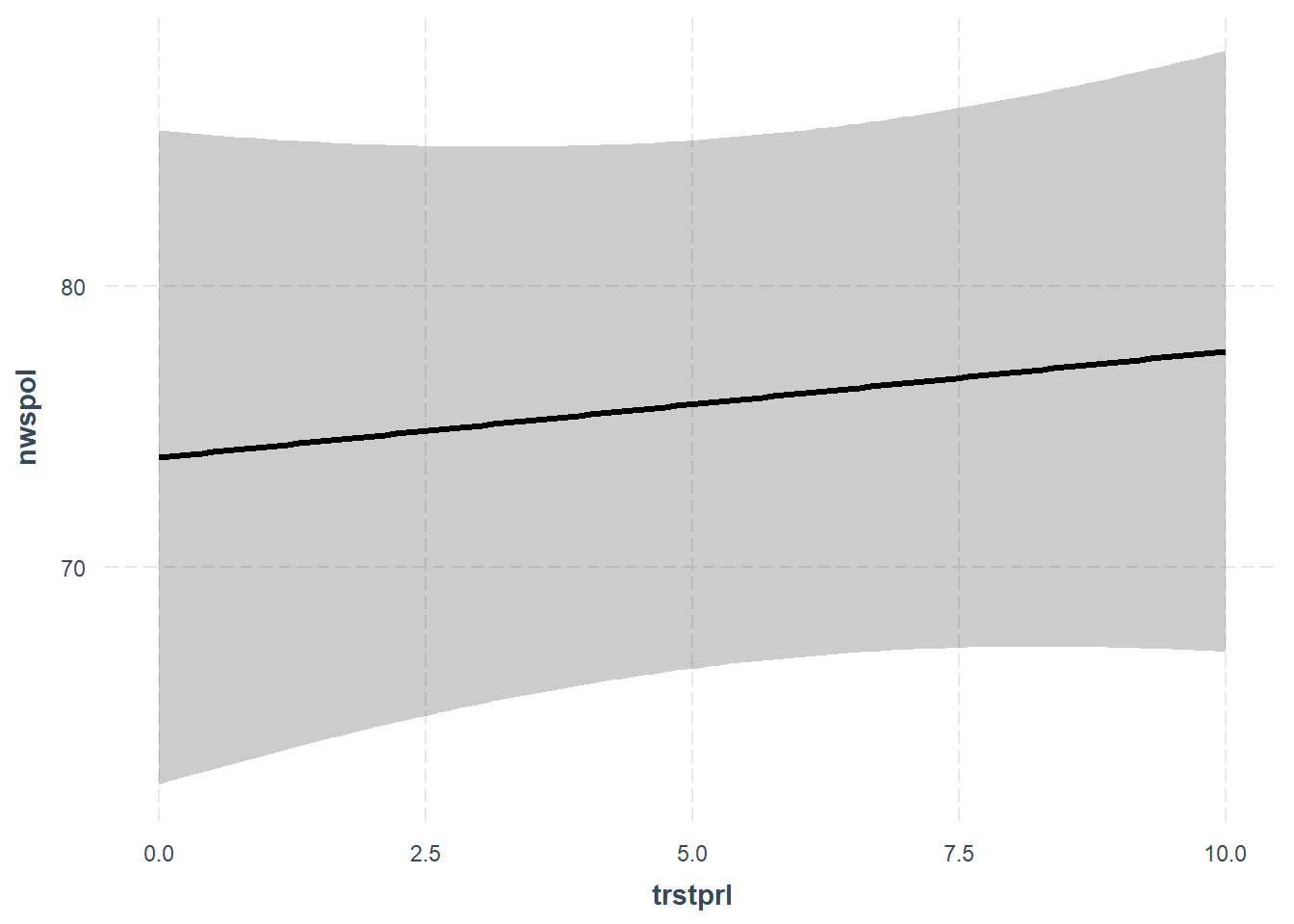

The error bars are very large, which makes sense because this was not a statistically significant relationship in the model.

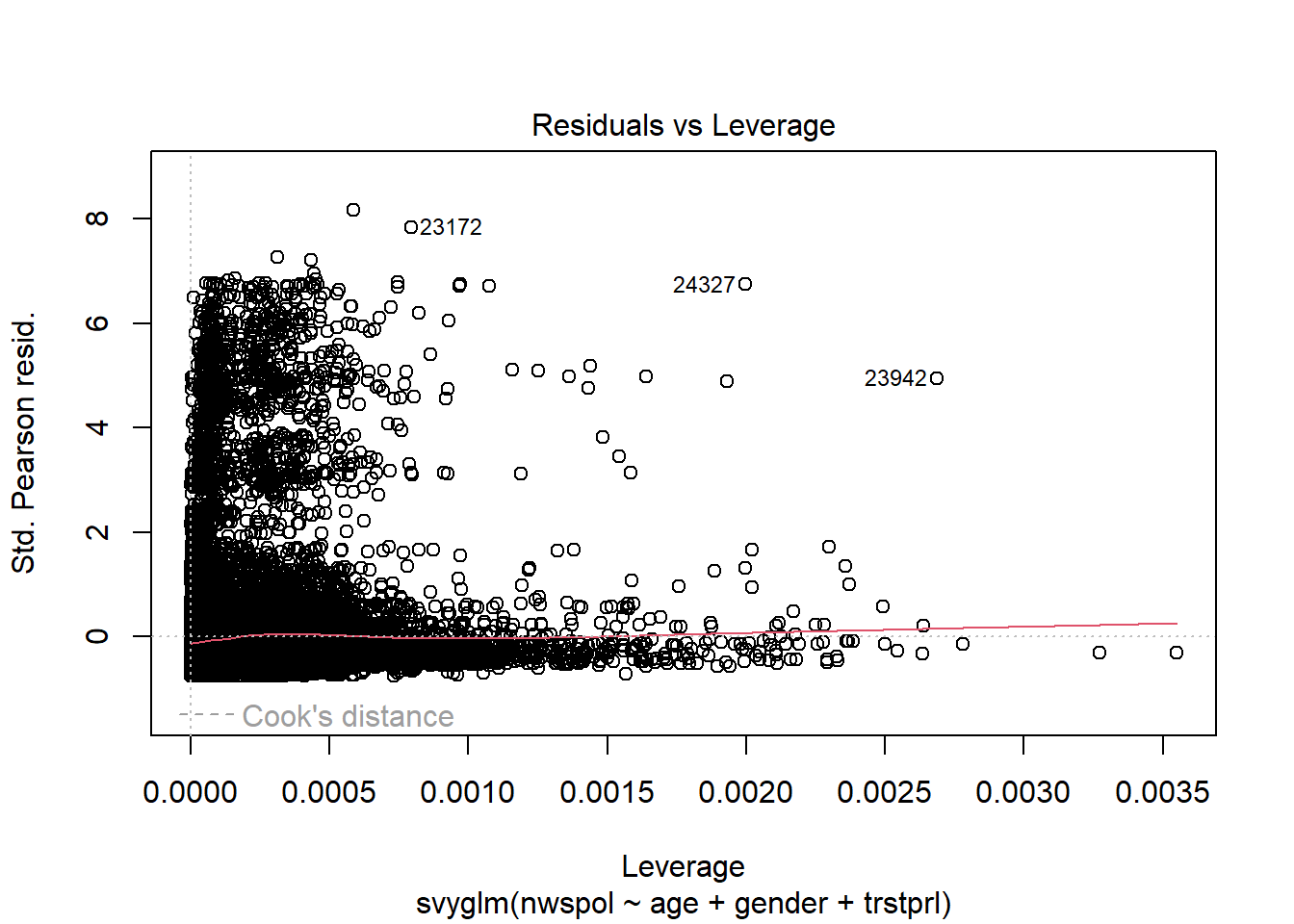
Calling plot on the data object provides a host of residuals plots.

Code

plot(m2)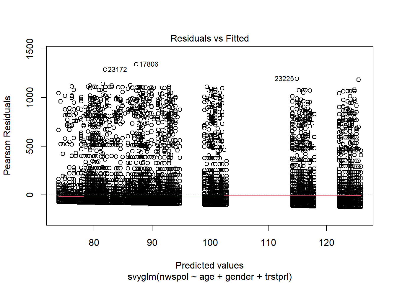

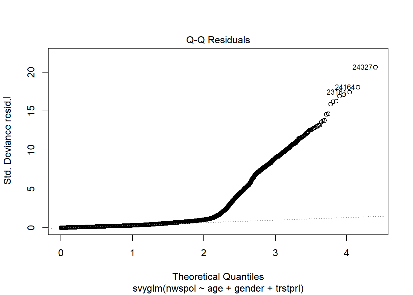
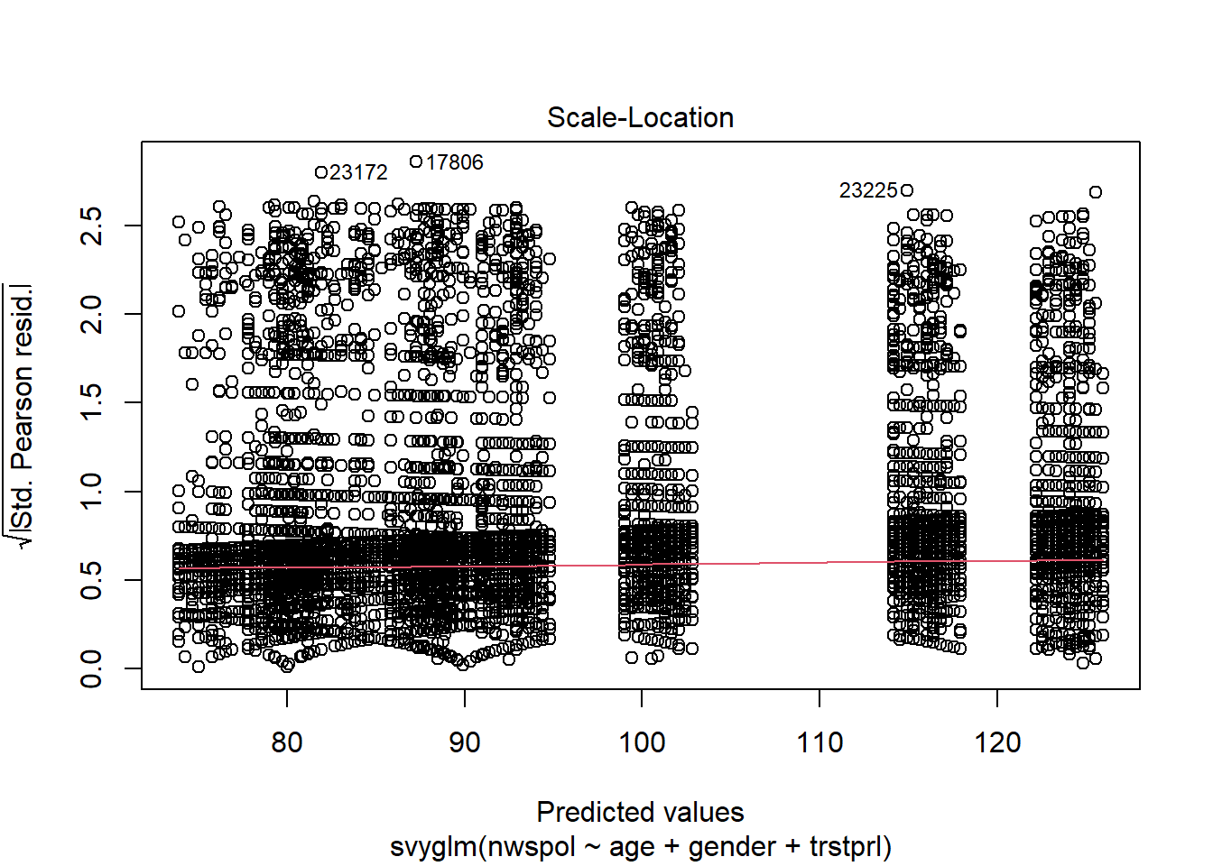
The qqplot indicates that the fit gets worse for the top quantiles.

The Scale-Location plot does not raise significant alarm bells for homoscedasticity.

Your turn!

Practice your own survey data analysis and extensions… There are many!

I hope these workshop materials were helpful in some way.